7  Simple Linear Regression

Packages Used

This chapter uses the following packages: ggplot2, ggdist, sjPlot, gridExtra, broom, performance, and the Lung function dataset.

The goal of linear regression is to describe the relationship between an independent variable X and a continuous dependent variable \(Y\) as a straight line.

Data for this type of model can arise in two ways;

• Fixed-\(X\): values of \(X\) are preselected by investigator
• Variable-\(X\): have random sample of \((X,Y)\) values

Both Regression and Correlation can be used for two main purposes:

• Descriptive: Draw inferences regarding the relationship
• Predictive: Predict value of \(Y\) for a given value of \(X\)

Simple Linear Regression is an example of a Bivariate analysis since there is only one covariate (explanatory variable) under consideration.

7.1 Example

Lung function data were obtained from an epidemiological study of households living in four areas with different amounts and types of air pollution. The data set used in this book is a subset of the total data. In this chapter we use only the data taken on the fathers, all of whom are nonsmokers (see PMA6 Appendix A for more details).

One of the major early indicators of reduced respiratory function is FEV1 or forced expiratory volume in the first second (amount of air exhaled in 1 second). Since it is known that taller males tend to have higher FEV1, we wish to determine the relationship between height and FEV1. We can use regression analysis for both a descriptive and predictive purpose.

• Descriptive: Describing the relationship between FEV1 and height
• Predictive: Use the equation to determine expected or normal FEV1 for a given height

ggplot(fev, aes(y=FFEV1, x=FHEIGHT)) + geom_point() + 
      xlab("Height") + ylab("FEV1") + 
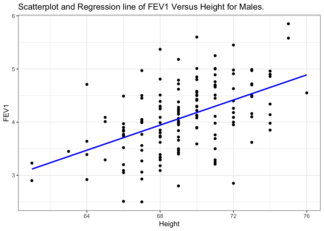
      ggtitle("Scatterplot and Regression line of FEV1 Versus Height for Males.") + 
      geom_smooth(method="lm", se=FALSE, col="blue") 

In this graph, height is given on the horizontal axis since it is the independent or predictor variable and FEV1 is given on the vertical axis since it is the dependent or outcome variable.

Interpretation: There does appear to be a tendency for taller men to have higher FEV1. The regression line is also added to the graph. The line is tilted upwards, indicating that we expect larger values of FEV1 with larger values of height.

Specifically the equation of the regression line is \[ Y = -4.087 + 0.118 X \]

The quantity 0.118 in front of \(X\) is greater than zero, indicating that as we increase \(X, Y\) will increase. For example, we would expect a father who is 70 inches tall to have an FEV1 value of

\[\mbox{FEV1} = -4.087 + (0.118) (70) = 4.173\]

If the height was 66 inches then we would expect an FEV1 value of only 3.70.

Caution on out of range predictions

To take an extreme example, suppose a father was 2 feet tall. Then the equation would predict a negative value of FEV1 (\(-1.255\)).

A safe policy is to restrict the use of the equation to the range of the \(X\) observed in the sample.

7.2 Mathematical Model

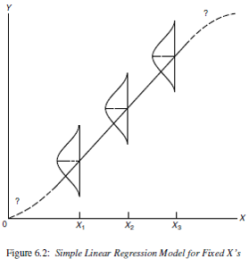
The mathematical model that we use for regression has three features.

1. \(Y\) values are normally distributed at any given \(X\)
2. The mean of \(Y\) values at any given \(X\) follows a straight line \(Y = \beta_{0} + \beta_{1} X\).
3. The variance of \(Y\) values at any \(X\) is \(\sigma^2\) (same for all X). This is known as homoscedasticity, or homogeneity of variance.

Mathematically this is written as:

\[ Y|X \sim N(\mu_{Y|X}, \sigma^{2}) \\ \mu_{Y|X} = \beta_{0} + \beta_{1} X \\ Var(Y|X) = \sigma^{2} \]

and can be visualized as:

Figure 6.2